Bucketing optimization in SQL to deal with skewed data (BigQuery example)

The 10x+ optimization that you may never tried

Introduction

Cloud data warehouses provide an excellent platform for handling large-scale data, allowing transformations at the terabyte scale to be processed in just minutes or even less, depending on the required operations.

Most platforms operate using a large number of small workers, enabling significant flexibility in hardware resources and scalability during processing, thereby maximizing parallelism. This approach generally works well, as the system often repartitions the input to align with your data size. However, these systems can struggle with skewed data, necessitating manual intervention to optimize performance.

Bucketing optimization (similar to salting) can significantly improve query run times.

For instance, below metrics are an example of the bucketing technique on skewed production data:

We’re getting close to a 18x run time speed up!
Let’s delve into the topic of skewed data, starting with the basics.

What’s skewed data?

First, let's define data skew: it refers to an imbalance in the distribution of data across various partitions, nodes, or workers in a distributed system. This imbalance can cause inefficiencies and performance issues, as some nodes or workers may be overloaded while others are underutilized. In extreme cases, it can even lead to out-of-memory errors.

We can identify three types of skew:

Data-Related Skew

This occurs when data is unevenly distributed across partitions or workers, often due to imbalanced input files.

Key-Related Skew

This happens when some keys (used in operations like joins or aggregations) are much more frequent than others.

Algorithm-Related Skew

This type arises when the processing logic creates hotspots by its design, which may also be influenced by the inputs.

We will briefly examine data-related skew and then focus on key-related skew. Algorithm-related skew is too specific for a general approach, though the bucketing strategy could be reused with an understanding of the data topology causing the skew.

Data skew

Example

Imagine your data is partitioned by day and then by customer. With 100 days and 100 customers, we would have 10,000 files. With 1,000 workers, it seems straightforward that each worker would process 10 files. However, what happens if one customer on one day has 1,000 times more data than the average?

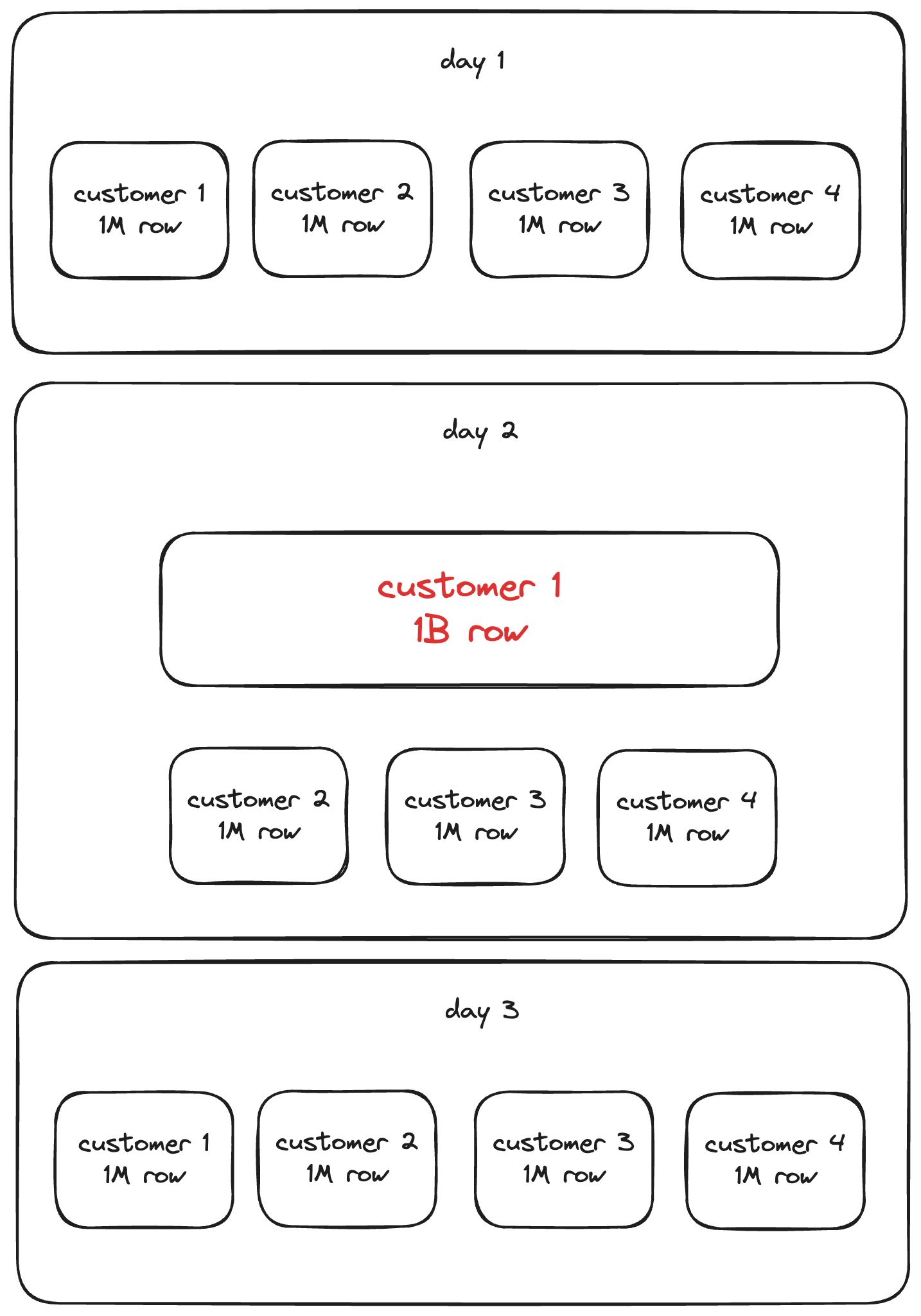
In this scenario, if it takes one minute to process an average file, the largest file would take 1,000 minutes, resulting in a job duration of more than 16 hours. If the data were balanced and all other files were around the average size, the workload would be similar to processing 11,000 files, which could be optimally handled in just 11 minutes!

Solution

To address this issue, you would typically try to balance the data at the partitioning level by adjusting the partitioning strategy or adding another level to further distribute the skewed data. This is not always straightforward, so data systems like BigQuery implement “repartitioning” steps to balance the partitions during processing. While this approach is transparent and efficient, it is not without cost: it requires a “data shuffle,” where rows are sent across available workers to balance the workload. It is generally assumed that most data warehouses can appropriately repartition data before storing it.

How to detect it ?

The most effective way to detect skew is by examining your table. We’ll assume that the table is partitioned and/or clustered (if it wasn’t, you wouldn’t have data skew as BigQuery would create balanced storage).

Consider the following table:

CREATE OR REPLACE TABLE
  my_gcp_project.my_dataset.my_skewed_table
PARTITION BY
  RANGE_BUCKET(id, GENERATE_ARRAY(0, 100, 1)) AS
SELECT
  *
FROM
  UNNEST([STRUCT(1 AS id, 10 AS views),
          STRUCT(1, 20),
          STRUCT(1, 30),
          STRUCT(1, 40),
          STRUCT(2, 50),
          STRUCT(2, 60),
          STRUCT(3, 70),
          STRUCT(3, 80),
          STRUCT(4, 90),
          STRUCT(4, 100)
        ])

Unless repartitioned, the file associated with id = 1 will be larger than those for other keys.

If your table schema is flat and balanced (i.e., it doesn’t contain arrays, and string fields are not skewed in length), the skew will be in the row count. Detecting it is as simple as performing a grouped query:

SELECT id, count(*) rows_count
FROM my_gcp_project.my_dataset.my_skewed_table
GROUP BY id
ORDER BY rows_count DESC

For small datasets, it's easy to identify skewed data by inspecting the top keys. However, for larger datasets, visualizing the actual distribution can be more informative. Drawing appropriate quantiles can be particularly helpful. Personally, I prefer splitting the data into 100 quantiles to understand the data distribution by percentage.

To achieve this, you can use the following query:

WITH skew_data_rows_count AS (
SELECT id, count(*) rows_count
FROM my_gcp_project.my_dataset.my_skewed_table
GROUP BY id
ORDER BY rows_count DESC
), quantiles AS (
SELECT APPROX_QUANTILES(rows_count, 99) quantiles_array
FROM skew_data_rows_count
)
SELECT row_number() over() pct, q as rows_count FROM quantiles, UNNEST(quantiles_array) q

As the chart indicates, 25% of the IDs are skewed (1 out of 4, as expected). Understanding the proportion and extent of skewed keys is crucial for determining how to bucket our data effectively.

Solving the data skew

If the data engine does not automatically unskew our data at storage time, we need to introduce bucketing. Let’s revisit the previous example.

We aim to create buckets that normalize the row count to the mean, which in this case is 2. Therefore, we want to distribute ID values into up to 2 buckets.

The easiest way to retrieve the mean is to use the following query:

WITH rows AS (
SELECT id,
       COUNT(*) AS rows_count
FROM my_gcp_project.my_dataset.my_skewed_table
GROUP BY ALL
)
SELECT
  CAST(PERCENTILE_CONT(rows_count, 0.5) OVER(PARTITION BY id) AS INT64) AS bucket_count
FROM
  rows
LIMIT 1

Then here’s how we can achieve the unskewed table creation:

CREATE OR REPLACE TABLE
  my_gcp_project.my_dataset.my_unskewed_table
PARTITION BY
  RANGE_BUCKET(id, GENERATE_ARRAY(0, 100, 1))
CLUSTER BY id, bucket
AS
(
WITH table_with_row_num AS (
    SELECT
        id,
        views,
        ROW_NUMBER() OVER (PARTITION BY id) AS row_num
    FROM `my_gcp_project.my_dataset.my_skewed_table`
)
SELECT
  id,
  views,
  CAST(CEIL(row_num / 2) AS INT64) AS bucket
FROM table_with_row_num)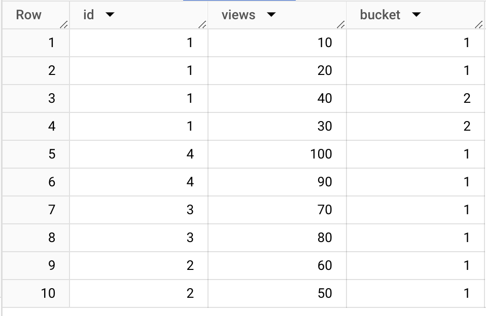

In this example, all distinct (id, bucket) tuples have a size of 2, ensuring balanced operations leveraging these tuples. However, this method may not universally improve the performance of all operations.

Performance

To illustrate the performance gain, let’s scale the dataset to 100M rows (~1.5 GB):

CREATE OR REPLACE TABLE
my_gcp_project.my_dataset.my_skewed_table
CLUSTER BY id
AS
(SELECT (CASE WHEN i*j < 1000000 THEN 1 ELSE CAST(i*j/10+1 AS INT64) END) as id,
 CAST(RAND()*10 AS INT64) views 
 FROM UNNEST(GENERATE_ARRAY(1, 1000000, 1)) i,
 UNNEST(GENERATE_ARRAY(1, 100, 1)) j)

We will unskew it with buckets of 100 rows each and compare a simple SUM operation on both tables:

SELECT id, APPROX_QUANTILES(views, 99) v
FROM {{ target_table }}
GROUP BY 1

Results

The first results are interesting:

• On the skewed table, we have:

  • Elapsed time: 8 sec

  • Slot time consumed: 9 min 24 sec

  • Bytes shuffled: 25.58 GB

• On the unskewed table, we have:

  • Elapsed time: 8 sec

  • Slot time consumed: 8 min 32 sec

  • Bytes shuffled: 25.46 GB

The results show a slight efficiency improvement in the unskewed table. Although the gains are modest and metrics are similar, this suggests that BigQuery may already optimize the data layout to some extent without further manual intervention.

So is it useless?

No, bucketing is not useless, especially for platforms that don’t automatically unskew your data. While the engine might rebalance data within a single dataset, it often cannot address key-related skew effectively (which is a great transition for the next part!).

Key-related skew

Key related skew is somehow the follow up issue when you have a data skew. It’s common to have a dimension on which we have a data skew. Then we need to join that skewed data with reference data to enrich it.

Example

Consider a scenario where the skewed data is the fact table, and we need to enrich it by joining it with a reference table. Extending the previous example:

In this case, customer 1’s data will require reference data by joining on the common “customer_id.” Often, the reference data is small enough to fit in memory on all executors, which is the most common way for data platforms to handle key-related skews. The system copies the reference table data to all executors and then evenly distributes the fact table data to perform the join.

However, in cases where both tables are large and cannot fit in memory, the system will perform a “smart join,” such as a hash join (where the join keys are hashed to distribute data on the same keys across executors). In our example, the rows for customer 1 will create a hotspot because they will be processed by a few executors that cache the reference data. This approach is efficient in terms of CPU time but results in a few workers handling significantly more operations than others.

Solution

The goal is to rebalance the data across more executors to improve job speed (in elapsed time), even if it is slightly less efficient overall. To achieve this, we can reuse the data skew solution: create multiple buckets for customers with many rows in the fact table. We then join both on the customer_id and the bucket. This prevents artificial bottlenecks because the (customer_id, bucket) tuples will have sizes limited to the buckets.

This increased bucketing can also improve aggregations. For instance, if you want to SUM a column, you can first SUM by (customer_id, bucket) and then aggregate these intermediate results by customer_id. This approach reduces the shuffle each executor needs to perform, as they can sum at their level and only shuffle the intermediate results for the final aggregation by customer_id.

How to detect it ?

Key-related skews are similar to data skews: if one of the tables involved in a join is skewed on the join key, you have a key-related skew situation.

Solving key-related skew

Assuming we have already created the unskewed table (my_gcp_project.my_dataset.my_unskewed_table) using the data skew solution, the join would initially look like this:

Then we need to reproduce bucketing on the reference table as well to have following setup:

To do so, we’re going to bucket the reference table as well as using the fact table bucket distribution and proceed with the actual join.

Let’s generate the reference table:

CREATE OR REPLACE TABLE
my_gcp_project.my_dataset.my_reference_table
CLUSTER BY id
AS
(SELECT i as id, ARRAY(SELECT AS STRUCT CONCAT("key ", j) AS k, CONCAT("value ", j) AS v FROM UNNEST(GENERATE_ARRAY(1, 1000)) j) my_large_reference_field
FROM UNNEST(GENERATE_ARRAY(1, 1000000, 1)) i)

Next, prepare the reference table with buckets:

CREATE OR REPLACE TABLE
my_gcp_project.my_dataset.my_reference_table_with_bucket
CLUSTER BY id, bucket
AS
(WITH
fact_table_bucket_distribution AS (
 SELECT id, MAX(bucket) bucket_count
 FROM my_gcp_project.my_dataset.my_unskewed_table
 GROUP BY id
)
SELECT id, my_large_reference_field, bucket
FROM my_gcp_project.my_dataset.my_reference_table
JOIN fact_table_bucket_distribution USING(id)
LEFT JOIN UNNEST(GENERATE_ARRAY(1, bucket_count)) as bucket
)

Finally, perform the join:

SELECT id, my_large_reference_field, views
FROM my_gcp_project.my_dataset.my_unskewed_table
JOIN my_gcp_project.my_dataset.my_reference_table_with_bucket USING(id, bucket)

This approach should result in a much faster operation. Although it might consume more slot time due to the preparation required to unskew the join, it can prevent queries from running into BigQuery’s timeout limit (6 hours), making it highly relevant in extreme cases.

Performance

To analyze the performance we’ll use (again) the 100M fact table that has ~1M keys.

Here’s the skewed tables join we’re using:

SELECT id, my_large_reference_field, views
FROM my_gcp_project.my_dataset.my_skewed_table
JOIN my_gcp_project.my_dataset.my_reference_table USING(id)

Then results are on another level:

• On the skewed tables, we have:

  • Elapsed time: 6 min 27 sec

  • Slot time consumed: 1 day 3 hr

  • Bytes shuffled: 2.68 TB

    

• On the unskewed tables, we have:

  • Elapsed time: 23 sec

  • Slot time consumed: 14 hr 56 min

  • Bytes shuffled: 2.67 TB

The ratio here is impressive: about 16x faster. It also performs better in terms of slot time, though not as dramatically as elapsed time.

What to notice about it? Well, as expected, the join is much faster! It’s even more visible if we look at the compute part of that step:

• For the skewed run

  • avg: 6090 (6.1 s)

  • max: 13140 (13 s)

• For the unskewed run

  • avg: 4763 (4.7 s)

  • max: 700995 (11.68 min)

So that solution is definitely working out as it enables us to get rid of the skew!

Another point to note is the slight reduction in keys for the unskewed run. As we created the my_reference_table_with_bucket table by joining with the actual keys from the fact table (of which only 95% are present), the reference table size for the join is slightly reduced. While this helps, the main reason for improved performance is the efficient processing of partitions using bucketing.

Conclusion

In this article, we focused on improving performance, particularly in terms of elapsed time rather than efficiency. Consequently, this strategy might not be suitable for every situation.

When to use the bucketing strategy? (all conditions apply)

• The skew is identified.

• The downstream queries are slow.

• No other simpler strategies apply (e.g., improving the filtering).

When to avoid the bucketing strategy?

• The performance gain is not worth the added complexity.

• Your team lacks strong SQL fundamentals to understand and maintain the optimization.

• Your platform lacks the tools to manage temporary tables and multiple transformations.

Although not emphasized much, intermediate transformations are not free. They usually have a less significant impact on elapsed time and slot time, but they should not be overlooked. However, it is unlikely that these transformations will be a deal-breaker.

You might not always benefit from that approach depending on how BigQuery is partitioning the work as well. I had cases where I couldn’t figure why BigQuery wouldn’t leverage more units of work to speed up the process.

Future Considerations

I wonder if this optimization could be automated by the underlying engines. It seems plausible but would likely require sufficient metadata to be precomputed on the stored data so that skews can be detected and anticipated at the query planning level. Please comment or reach out if you know of any systems that can perform as well without manual optimizations. Ultimately, the goal is to reduce the mental overhead for end users, thereby improving readability and maintainability while achieving performance gains.

---

🎁 If this article was of interest, you might want to have a look at BQ Booster, a platform I’m building to help BigQuery users improve their day-to-day.

Also I’m building a dbt package dbt-bigquery-monitoring to help tracking compute & storage costs across your GCP projects and identify your biggest consumers and opportunity for cost reductions. Feel free to give it a go!

---

If you’re interested in working on high scale projects, at the time of writing, we’ve few openings at Teads. For instance, we’re looking for an engineering director, senior/staff software engineers (mostly full stack), senior data scientists and salesforce senior software engineers in Montpellier (France).

---

And don’t hesitate to share the post!